Measuring Bandwidth and Round-Trip Time of a TCP Connection inside the Application Layer
Recently, I had to measure the bandwidth and round-trip time of different simultaneous TCP connections in order to estimate optimal traffic distributions over different interfaces. That’s why in this post I want to cover how to measure the goodput (i.e., the application level throughput) and round-trip time of a TCP connection inside the application layer. We will measure both metrics while we download a file via HTTP (since HTTP is implemented on top of TCP).
Round-Trip Time
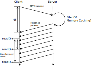
In order to estimate the round-trip time we have to measure the time that goes by between the client sending the first byte of a request to the server and receiving the first byte of the response from the server (as shown in the figure above). This technique does not take into account the time necessary on the server to process the request until sending the first byte of the response. Further, depending on the server hardware and configuration this processing time differs from machine to machine. For instance a server that uses resource memory caching will, in most cases have a lower processing time than a server without caching, since reading a resource from disk comes with a huge overhead compared to reading from memory. Luckily, this processing delay is usually comparatively much smaller than the link propagation delay and can thus be neglected.
In case we have multiple round-trip time estimates (several download rounds), we need to combine them to one fair estimate. The TCP layer also estimates the round-trip time (for retransmission purposes) using the weighed moving average. We could do the same on an application layer.
For each obtained round-trip time value \(rtt\) we estimate the overall \(\overline{rtt}\) using a weighed moving average:
\[\overline{rtt} = 0.8 \cdot \overline{rtt} + 0.2\cdot rtt\]By doing so, we give less importance to extreme outliers. Here is some corresponding code in c:
Bandwidth
There are some very important core thoughts we have to talk about first.
The period of time over which we measure
In general, when measuring the bandwidth of a TCP connection, it is very important to remember that all the different TCP flavors come with a slow-start algorithm. This means that a TCP connection initially transmits very few packets and over time increases the number of transmitted packets until a transmission error occurs. By doing so, TCP avoids network congestion better than other protocols such as UDP. For us, this means that the time over which we measure needs to be long enough for TCP to get close to the maximum transmission rate of the channel. In this example we choose to repeatedly download a 1M file.
Initial bursts and the start time
In general, the bandwidth is calculated as a number of bytes divided by the time it took to receive them, which means we need to find a start and end time to determine this time interval. The end time can be determined quite intuitively - simply use the timestamp of the last socket.read() call.
The start time on the other hand is a little more difficult to determine exactly. One way the estimation could be performed is by first saving the timestamp of the first socket.read() event and counting the number of bytes read since then. On every further socket.read() call we divide the total number of bytes since the beginning of the response by the time passed since the first read event. An important issue we have to consider is that the first read call might return more bytes in a short amount of time than the following read calls. This is due to the fact that we do not measure directly on the link the arrival of the packets, but instead measure when the packets arrive in our application layer. Until the first bytes are processed and ready for the application layer to be read, a lot of bytes might already be buffered in the lower layers. This leads to a burst of data in the beginning once all the necessary structures are setup on all the other layers. In another implementation in order to avoid this burst falsifying our estimate, we simply neglect the first samples of the first read operations and use the timestamp of a later socket.read() call as the starting time.
In the end of this post I add a program, that uses both ways to estimate the bandwidth - by running this program you can easily witness the difference between them.
The harmonic mean
A single network measurement can be highly unreliable due to general network variations, which is why we measure several times over a certain period (e.g., until the complete file is downloaded). The harmonic mean can then be used, because it mitigates the impact of such large outliers and can be easily computed. Consequently, the harmonic mean is a very good way to combine these measurement values into one general average bandwidth estimate.
Given a series of bandwidth measurements \(R(t)\), where \(t=0,1,2,\cdots, n-1\), the harmonic mean \(\overline{R}\) is calculated as:
\[\overline{R} = \frac{n+1}{\frac{n}{\overline{R}} + \frac{1}{R(n+1)}}\]Here is an example implementation for the harmonic mean in c:
Putting it all together
Now that we have discussed everything, here is a program that downloads a file several times and measures the round-trip time and bandwidth. For convenience, this program uses HTTP/1.1 (that way it is much easier to deploy a testing resource on a server). Since HTTP runs on top of TCP, we still have a valid TCP socket to measure the metrics. One might argue, that HTTP introduces an extra overhead which falsifies the results. Still, when downloading a static resource the propagation delay between client and server should be much higher than this overhead; thus we can neglect it.
The bandwidth is measured in two ways:
- First, by using the first
socket.read()timestamp as the start time. - Second, by using a later subsequent
socket.read()timestamp as the start time (to avoid bursts and slow-start falsifying the estimate).
I wrote a simple command line tool which applies these measurement methods: Check out tcp-metrics.
I use disqus as a comment system. If you click on the following button, then the disqus comment system will load in your browser and you agree to the disqus privacy policy. To delete your data from disqus you can contact their support team directly.